Linux schedulers are built on carefully tuned heuristics. However, they are static and apply the same rules across all workloads. Modern systems run a wide range of workloads, from latency-sensitive tasks to long and heavy workloads. A single, fixed scheduling policy cannot optimally serve all of these use cases. Sometimes, this leads to high latency or unfair resource allocation under certain workloads. My goal was to move beyond this limitation by enabling the scheduler to learn from runtime behavior.
What exactly is a scheduler?
A process scheduler in an operating system decides which process to run next. Yet my computer appears to run Spotify, Valorant, and 20 Chrome tabs all at the same time. If that’s the case, why do we need a scheduler at all? The answer lies in how modern CPUs share time among competing processes. Even on multi-core systems, resources are finite, and the scheduler must constantly decide who gets the CPU and for how long.
You can think of this process as a game of "Overcooked", where each incoming task is a new order and each player represents a CPU core. Despite having only a limited number of players, the kitchen can handle a large number of orders through proper scheduling, deciding what each player should work on at the right time so that no customer waits too long. In the same way, a scheduler must ensure that all tasks in the runqueue are completed before their deadlines expire.
 Credits: team17.com/games/overcooked
How does Linux schedule processes?
Linux uses the Completely Fair Scheduler (CFS) to schedule tasks, prioritizing fairness rather than relying solely on static priorities. CFS ensures that each task receives CPU time and is not starved. Each process is assigned a virtual runtime (vruntime), which indirectly represents the amount of processor time it has consumed relative to other tasks in the runqueue (more on this later). When selecting the next task to run, CFS chooses the task with the smallest virtual deadline, calculated based on its vruntime. This scheduling approach is derived from the Earliest Deadline First (EDF) algorithm and is implemented in the Linux kernel as Earliest Eligible Virtual Deadline First (EEVDF). This design ensures that no process is unfairly starved of CPU time. At a high level, CFS sounds simple, but its behavior is driven by several carefully designed mechanisms. Understanding how vruntime, weights, and virtual deadlines interact is key to understanding how Linux schedules processes in practice. Now that we know how CFS works on high level, let's dive deeper into the code.
When a new task is created, it is assigned the minimum vruntime among all tasks currently in the runqueue. But why the minimum? If vruntime represents the amount of processing time a task has consumed, shouldn’t it start at zero?
The reason for this choice is to keep the scheduler fair. Consider a scenario where task A has been running for a long time and is the only task in the runqueue. If a new task B is initialized at this point and assigned a vruntime of zero, task A would not be scheduled again until task B has consumed the same amount of processor time. This would effectively cause task A to starve. To avoid this, task B is instead assigned the minimum vruntime in the runqueue, which, in this case, is the vruntime of task A.
How is this minimum vruntime calculated? In the Linux scheduler, the runqueue’s min_vruntime is updated on every scheduler tick. At each tick, CFS examines the task with the smallest vruntime and compares it against the current min_vruntime. If the task’s vruntime exceeds the stored minimum, min_vruntime is changed to this value.
Oversimplified version of kernel code to calculate min_vruntime
1static void update_min_vruntime(struct cfs_rq *cfs_rq)
2{
3    struct sched_entity *se = __pick_root_entity(cfs_rq); // Lowest vruntime task
4    struct sched_entity *curr = cfs_rq->curr;             // Currently running task
5
6    u64 vruntime = cfs_rq->min_vruntime;
7
8    // Compare against the smallest vruntime entity
9    if (se) {
10        if (!curr)
11            vruntime = se->min_vruntime;
12        else
13            vruntime = min_vruntime(vruntime, se->min_vruntime);
14    }
15
16    u64 new_min_vruntime = cfs_rq->min_vruntime;
17    s64 delta = (s64)(vruntime - new_min_vruntime);
18
19    if (delta > 0) {
20        avg_vruntime_update(cfs_rq, delta);
21        cfs_rq->min_vruntime = vruntime;
22    }
23}
24
Now that we have the vruntime for each task and themin_vruntime, we can begin ordering tasks in the runqueue. The runqueue is implemented as a red-black tree, allowing O(log n) insertion and deletion. Tasks are ordered based on their virtual deadlines rather than raw runtime.
These virtual deadlines are calculated using a task’s vruntime and its NICE value, which allows users to manually prioritize or deprioritize tasks. The virtual deadline is computed as follows:
Here, NICE_0_WEIGHT represents the scheduling weight associated with a NICE value of 0. Similarly, task_weight is derived from the custom NICE value provided by the user. The slice parameter defines the default duration for which a task is allowed to execute and is set to 700,000 by default unless overridden.
CFS selects the task with the lowest virtual deadline from the runqueue and begins executing it. The task continues to run until its deadline exceeds that of the next task in the runqueue and it has executed for at least the default slice duration (700,000 ns). At this point, the current state of the CPU while running this task is stored in a struct and a new task is scheduled to run.
Oversimplified version of kernel code to calculate deadline and preempt
1void update_curr(struct cfs_rq *rq)
2{
3    // Current running task
4    struct sched_entity *task = rq->curr;
5
6    if (!task)
7        return;
8
9    // Time the task just ran
10    u64 delta_exec = get_execution_time(task);
11    if (delta_exec == 0)
12        return;
13
14    // Advance virtual runtime based on priority
15    task->vruntime += (delta_exec * NICE_0_LOAD) / task->load.weight;
16
17    // Recompute the task's virtual deadline
18    task->deadline = task->vruntime + task->slice;
19
20    // Advance the runqueue's minimum vruntime
21    rq->min_vruntime = min(rq->min_vruntime, task->vruntime);
22
23    // Preempt if another task now has an earlier deadline
24    if (task->deadline > next_earliest_deadline(rq))
25        schedule_next_task();
26}
27
28static inline u64 calc_delta_fair(u64 delta_exec, struct sched_entity *se)
29{
30    u64 task_weight = se->load.weight;
31
32    /* If task has default priority, no scaling is needed */
33    if (task_weight == NICE_0_LOAD)
34        return delta_exec;
35
36    /* Scale execution time based on task priority */
37    return (delta_exec * NICE_0_LOAD) / task_weight;
38}
39
Adaptive Learning
Up to this point, we have seen how Linux relies on fixed rules to balance fairness and responsiveness. In practice, however, different workloads place very different demands on the scheduler, often requiring distinct scheduling strategies for optimal performance. This raises a natural question: instead of relying on fixed rules, can the scheduler learn to adapt to changing workloads and make smarter scheduling decisions?
As we saw earlier, the virtual deadline of a task plays a crucial role in determining which task runs next. But what if, instead of relying on fixed heuristics, we could use learning-based methods to influence this virtual deadline?
In the current design, the slice term is the same for every task and is set to 700,000 ns by default. Rather than keeping this value fixed, we can use reinforcement learning to adapt the slice dynamically based on observed workload behavior and system conditions. Metrics such as a task’s wait time, and burst time can be used to inform these decisions.
Proximal Policy Optimization (PPO)
Even though scheduling decisions are discrete and made periodically, the inputs to the scheduler such as burst time and wait time are continuous. For this case, a reinforcement learning algorithm like Proximal Policy Optimization (PPO) is well suited, as it can operate over continuous state spaces while producing stable policy updates.
On a high level, it is a RL algorithm with an actor and a critic. The actor or the policy interacts with the environment and receives some reward from the environment and the critic evaluates how good the action taken is. This separation allows the policy to improve its decisions while relying on the critic for stable and low-variance learning signals. If you are interested in learning more about PPO, this is the original PPO paper.
The Agent
To make scheduling decisions, I use a set of task-level and queue-level metrics as inputs to the agent. These include a task’s last wait time, average wait time, last burst time, and average burst time, as well as the runqueue’s average wait time and average burst time. The task-level metrics allow the agent to make decisions that are responsive to individual tasks, while the queue-level metrics ensure that these decisions account for overall system behavior and do not unfairly ignore other runnable tasks.
As discussed earlier, I want to work on changing the default task time slice of 700,000 ns. Hence, the action space starts at 70,000 ns (one tenth of the default) to enable shorter execution windows and lower virtual deadlines for latency-sensitive tasks, and extends to 1,120,000 ns in increments of 105,000 µs. The policy outputs a discrete probability distribution over these slice values, from which a slice is sampled and assigned to the task at each scheduling decision.
The next step was designing the reward function, a critical component that directly shapes the agent’s behavior. The primary objective was to minimize task wait times while avoiding excessive burst fragmentation and unnecessary context switches. To achieve this, the reward function was designed to favor low wait times, longer burst execution, and fewer context switches.
A naive approach would be to define the reward solely based on the current task’s most recent metrics. However, such a formulation would result in a greedy policy that prioritizes short-term gains for the current task, potentially leading to starvation of other runnable tasks. To prevent this, I used runqueue-level signals, specifically average wait time and turnaround time, into the reward formulation. As a result, the reward function encourages minimizing overall context-switch overhead and average wait time while maximizing average turnaround time across the runqueue.
I use a neural network as the policy to make scheduling decisions based on the observed state. The policy network consists of two hidden layers with tanh activation functions, followed by a softmax output layer that produces a probability distribution over the discrete action space. The first hidden layer contains 50 nodes, and the second contains 70 nodes. This relatively small architecture was chosen to minimize latency and memory overhead, which are critical constraints when deploying a model inside the kernel.
The Simulator
At this point, the next challenge was deciding where to train the RL agent. Training directly in the kernel was impractical, as it would require manually extracting logs to userspace, training there, and repeatedly updating the kernel with new parameters. To simplify this process and enable faster iteration, I decided to build a custom scheduler simulator in Python. The simulator attempts to replicate Linux’s CFS as closely as possible, with each subroutine and scheduling decision implemented to mirror the kernel logic. I also implemented a custom version of PPO, using separate neural networks for the actor and critic, and integrated it directly with the simulator. The code for this simulator can be found here.
To train the agent, I created a set of synthetic task types, including long-lasting CPU-heavy tasks, tasks with short CPU bursts, and tasks with short I/O bursts. Multiple instances of these tasks were periodically added to the simulator, forming a dynamic workload. At each scheduling decision, the RL agent selected a time slice for the currently running task and trained on the resulting system behavior.
After training, I evaluated the adaptive scheduler against the stock CFS implementation in my simulator. Both schedulers were tested using identical workloads, with tasks having the same execution times and burst characteristics. I then compared their average wait times and burst times to assess the impact of the learned scheduling policy. The results are shown below.
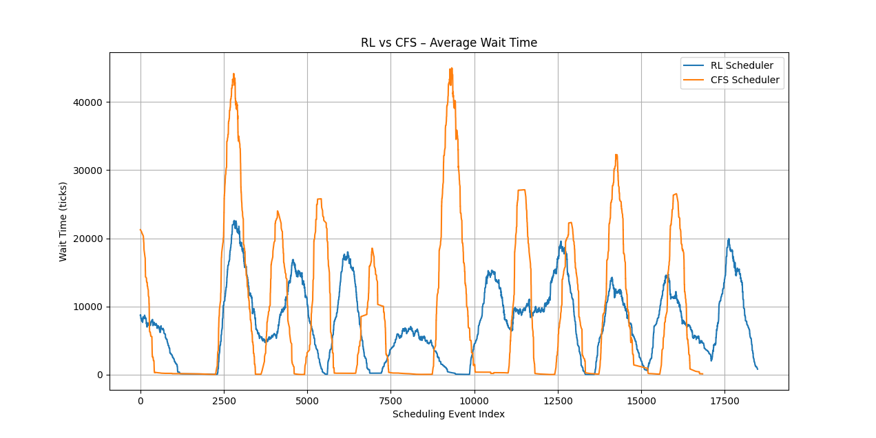 Adaptive Scheduler vs Stock CFS Scheduler wait times
The graphs above show the wait-time distributions for the stock CFS scheduler and the adaptive RL-based scheduler under identical workloads. The adaptive scheduler consistently maintains lower average wait times, with individual task wait times remaining within a narrow range. In contrast, the stock CFS scheduler exhibits significantly higher variance, with pronounced spikes indicating extreme wait times for certain tasks.
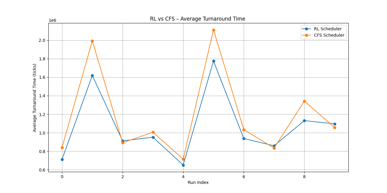 Adaptive Scheduler vs Stock CFS Scheduler turnaround times
This graph shows the average turnaround time across the ten workloads evaluated. The adaptive scheduler outperforms the stock CFS scheduler in seven out of ten cases, indicating a consistent improvement in scheduling decisions under these workloads.
Kernel Policy Integration
Now that a working and trained policy is in place, the next step is to integrate it into the Linux kernel. However, this task is far from straightforward. In userspace, training and experimentation benefited from high-level tools such as Python, NumPy, and various machine learning libraries, which make implementing and iterating on neural network policies relatively easy. In contrast, deploying the same policy inside the kernel requires reimplementing it in C under strict resource and performance constraints.
The first and most significant constraint was the lack of floating-point support in kernel space, unless floating-point registers are explicitly saved and restored, an approach that is both complex and costly. To address this, I adopted a Q-format fixed-point representation, where a fixed number of bits encode the integer portion of a value and the remaining bits represent the fractional component. However, this change introduced additional complexity, as all arithmetic operations, including multiplication and addition, had to be reimplemented to correctly support the chosen fixed-point format.
I began by converting all of the trained weights and biases for the policy neural net to Qn.32. However, I think the level of precision for Qn.32 might have been an overkill. After this, I had to implement matrix multiplication, tanh, softmax and other helper functions for Qn.32 in C. The codes for which can be found below:
C code to convert to Qn.32 (Q32.32 in particular)
1static inline q32_32 q32_from_int(s64 x){
2    __int128 t = (__int128)x << Q; return (q32_32)sat_s64(t);
3}
Matrix Multiplication
1static inline q32_32 qmul_q32_32(q32_32 a, q32_32 b) {
2    __int128 p = (__int128)a * (__int128)b;
3    if (p >= 0) p += (__int128)1 << (Q - 1); else p -= (__int128)1 << (Q - 1);
4    p >>= Q;
5    return (q32_32)sat_s64(p);
6}
7
8void nn_gemm_q32(const q32_32 *w, const q32_32 *x, const q32_32 *b, q32_32 *y, int rows, int cols) {
9    for (int i = 0; i < rows; i++) {
10        __int128 acc = 0;
11        const q32_32 *wi = w + (size_t)i * cols;
12        for (int j = 0; j < cols; j++) acc += (s64)qmul_q32_32(wi[j], x[j]);
13        if (b) acc += b[i];
14        y[i] = (q32_32)sat_s64(acc);
15    }
16}
Tanh calculation
1#define ONE_Q ((q32_32)1 << Q)
2
3void nn_tanh_q32(q32_32 *v, int n) {
4    for (int i = 0; i < n; i++) {
5        s64 x = v[i];
6        if (x > (s64)(4 * ONE_Q)) v[i] = ONE_Q;
7        else if (x < (s64)(-4 * ONE_Q)) v[i] = -ONE_Q;
8        else {
9            s64 x2 = qmul_q32_32((q32_32)x, (q32_32)x);
10            s64 num = x * ((s64)27 * ONE_Q + x2);
11            s64 den = ((s64)27 * ONE_Q) + (3 * x2);
12            v[i] = (q32_32)(num / den);
13        }
14    }
15}
Softmax Calculation
1static inline q32_32 qexp_q32_32(q32_32 x) {
2    const q32_32 MIN_X = -(8 * ONE_Q);
3    if (x > 0) x = 0;
4    if (x < MIN_X) x = MIN_X;
5    q32_32 c1 = ONE_Q, c2 = ONE_Q, c3 = ONE_Q >> 1, c4 = ONE_Q / 6, c5 = ONE_Q / 24, c6 = ONE_Q / 120;
6    q32_32 y = c6;
7    y = qmul_q32_32(y, x) + c5;
8    y = qmul_q32_32(y, x) + c4;
9    y = qmul_q32_32(y, x) + c3;
10    y = qmul_q32_32(y, x) + c2;
11    y = qmul_q32_32(y, x) + c1;
12    return y;
13}
14
15void nn_softmax_q32(const q32_32 *logits, q32_32 *probs, int n) {
16    s64 max = logits[0];
17    for (int i = 1; i < n; i++) if (logits[i] > max) max = logits[i];
18
19    q32_32 exps[OUTPUT_SIZE];
20    u64 sum = 0;
21    for (int i = 0; i < n; i++) {
22        q32_32 z = (q32_32)((s64)logits[i] - max);
23        q32_32 e = qexp_q32_32(z);
24        exps[i] = e;
25        sum += (u64)e;
26    }
27    if (!sum) { /* extremely defensive; should not happen */
28        for (int i = 0; i < n; i++) probs[i] = 0;
29        return;
30    }
31    for (int i = 0; i < n; i++) {
32        u64 q = mul_u64_u64_div_u64((u64)exps[i], (u64)ONE_Q, (u64)sum);
33        probs[i] = (q32_32)(s64)q;
34    }
35}
Forward Pass Neural Net Policy
1void forward(const q32_32 input[INPUT_SIZE]) {
2    nn_gemm_q32(&W1[0][0], input, B1, A1, HIDDEN_LAYER_1_SIZE, INPUT_SIZE);
3    nn_tanh_q32(A1, HIDDEN_LAYER_1_SIZE);
4    nn_gemm_q32(&W2[0][0], A1, B2, A2, HIDDEN_LAYER_2_SIZE, HIDDEN_LAYER_1_SIZE);
5    nn_tanh_q32(A2, HIDDEN_LAYER_2_SIZE);
6    nn_gemm_q32(&W3[0][0], A2, B3, NN_OUTPUT, OUTPUT_SIZE, HIDDEN_LAYER_2_SIZE);
7}
8
Each forward pass of the policy network takes approximately 15 µs. If an RL decision were made every time a task was enqueued, this overhead would accumulate quickly and significantly impact scheduling latency. To mitigate this cost, I chose to evaluate the policy for each task at most once every 1 ms. As a result, a task retains the same time slice for the duration of this 1 ms window, regardless of how many times it is enqueued, and is assigned a new slice only when the interval expires.
Results
After successfully integrating the policy into the Linux kernel and resolving numerous implementation issues, I was able to run the adaptive scheduler stably in kernel space. I then evaluated the adaptive scheduler alongside the stock CFS scheduler using identical workloads. The following table summarizes the observed results.
| Scheduler Type | Average Burst Time | Average Wait time |
|---|---|---|
| Stock CFS | 0.385 ms | 11.06 ms |
| RL Scheduler | 0.419 ms | 13.43 ms |
While the adaptive scheduler exhibits a slightly higher average wait time compared to stock CFS, this behavior is consistent with the reward formulation used during training. The reward function explicitly balances wait time reduction against longer burst execution and fewer context switches, prioritizing overall scheduling efficiency rather than minimizing wait time alone. As a result, the adaptive scheduler accepts a modest increase in wait time in exchange for improved burst behavior and reduced context-switch overhead.
Conclusion
Although the adaptive scheduler produced encouraging results, there remains significant potential for further optimization. In particular, training the policy directly within the kernel, rather than relying on an external simulator, could allow the agent to better capture real-world scheduling dynamics and hardware effects. Overall, this project deepened my understanding of how learning-based algorithms can be integrated into low-level systems such as the Linux kernel. Looking ahead, similar techniques could be extended to implement more aggressive scheduling policies, such as shortest job first (SJF) by appropriately redefining the reward function and adjusting the policy architecture to suit specific use cases.
